Masks

Here we show the effects of the type of filter to use in the Mask task.

Method linear

Theory

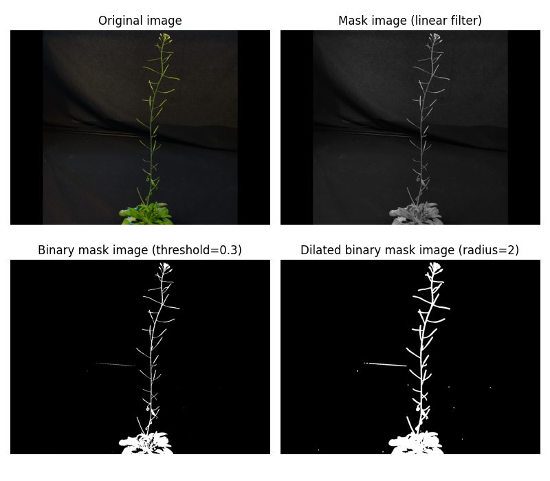
The equation for the linear filter method ($LF$) is as follows: $LF= c_r*R + c_g*G + c_b*B$, with $c_r$, $c_g$ & $c_b$ a coefficient in $[0., 1.]$ to apply to the corresponding channel.

Then we apply a high-pass threshold to binarize the image and create a mask locating the plant in the image. Finally, we use a binary dilation to enlarge the masked area.

Example & code

Here is an example of what the linear filter does when used in combination with a binarization step and a dilation step, as in the Masks task:

The source code for this figure is as follows:

import matplotlib.pyplot as plt
from imageio.v3 import imread
from plant3dvision import test_db_path
from plant3dvision.proc2d import linear, dilation
path = test_db_path()
img = imread(path.joinpath('real_plant/images/00000_rgb.jpg'))
rgb_coefs = [0.1, 1., 0.1]
filter_img = linear(img, rgb_coefs)  # apply `linear` filter
threshold = 0.3
mask = filter_img > threshold  # convert to binary mask using threshold
radius = 2
dilated_mask = dilation(mask, radius)  # apply a dilation to binary mask
fig, axes = plt.subplots(2, 2, figsize=(8, 7))
axes[0, 0].imshow(img)
axes[0, 0].set_title("Original image")
axes[0, 1].imshow(filter_img, cmap='gray')
axes[0, 1].set_title("Mask image (linear filter)")
axes[1, 0].imshow(mask, cmap='gray')
axes[1, 0].set_title(f"Binary mask image (threshold={threshold})")
axes[1, 1].imshow(dilated_mask, cmap='gray')
axes[1, 1].set_title(f"Dilated binary mask image (radius={radius})")
[ax.set_axis_off() for ax in axes.flatten()]
plt.tight_layout()

Important

Pay attention to the values used for rgb_coefs, threshold and dilation.

Method excess_green

Theory

This filter was published in: Woebbecke, D. M., Meyer, G. E., Von Bargen, K., & Mortensen, D. A. (1995). Color indices for weed identification under various soil, residue, and lighting conditions. Transactions of the ASAE, 38(1), 259-269.

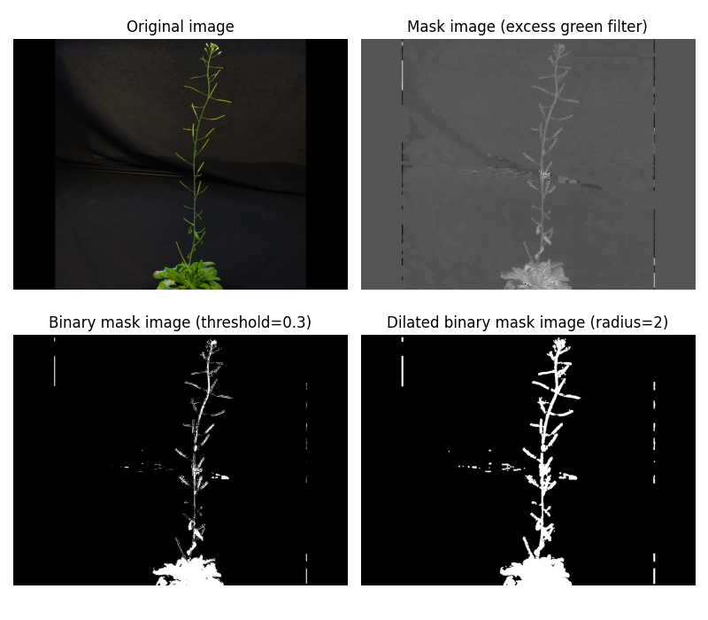
The equation for the excess green method ($EG$) is as follows: $EG= 2*g-r-b$, with:

• $r = R/(R+G+B)$
• $g = G/(R+G+B)$
• $b = B/(R+G+B)$
• Then we apply a high-pass threshold to binarize the image and create a mask locating the plant in the image. Finally, we use a binary dilation to enlarge the masked area.

Example & code

Here is an example of what the excess_green filter does when used in combination with a binarization step and a dilation step, as in the Masks task:

The source code for this figure is as follows:

import matplotlib.pyplot as plt
from imageio.v3 import imread
from plant3dvision import test_db_path
from plant3dvision.proc2d import excess_green, dilation
path = test_db_path()
img = imread(path.joinpath('real_plant/images/00000_rgb.jpg'))
filter_img = excess_green(img)  # apply `excess_green` filter
threshold = 0.3
mask = filter_img > threshold  # convert to binary mask using threshold
radius = 2
dilated_mask = dilation(mask, radius)  # apply a dilation to binary mask
fig, axes = plt.subplots(2, 2, figsize=(8, 7))
axes[0, 0].imshow(img)
axes[0, 0].set_title("Original image")
axes[0, 1].imshow(filter_img, cmap='gray')
axes[0, 1].set_title("Mask image (excess green filter)")
axes[1, 0].imshow(mask, cmap='gray')
axes[1, 0].set_title(f"Binary mask image (threshold={threshold})")
axes[1, 1].imshow(dilated_mask, cmap='gray')
axes[1, 1].set_title(f"Dilated binary mask image (radius={radius})")
[ax.set_axis_off() for ax in axes.flatten()]
plt.tight_layout()

Important

Pay attention to the values used for threshold and dilation.