Crops Insights Pipeline

Generating Orthomosaic Image

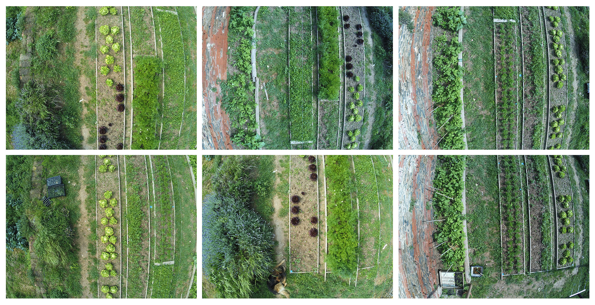
For the scope of this application, a rigorous system of collecting photographs of the fields was set, representing a first set of data to process; also to test different strategies of automatic navigation paths, by sending the same waypoints to the drones and to cable-bot. This set of instructions are basically following the rules of sweeping the entire area to then transform the data into an orthomosaic image which covers the whole crop. It’s important that the images have around 50% to 70% vertical overlap and around 30% overlap on sides.

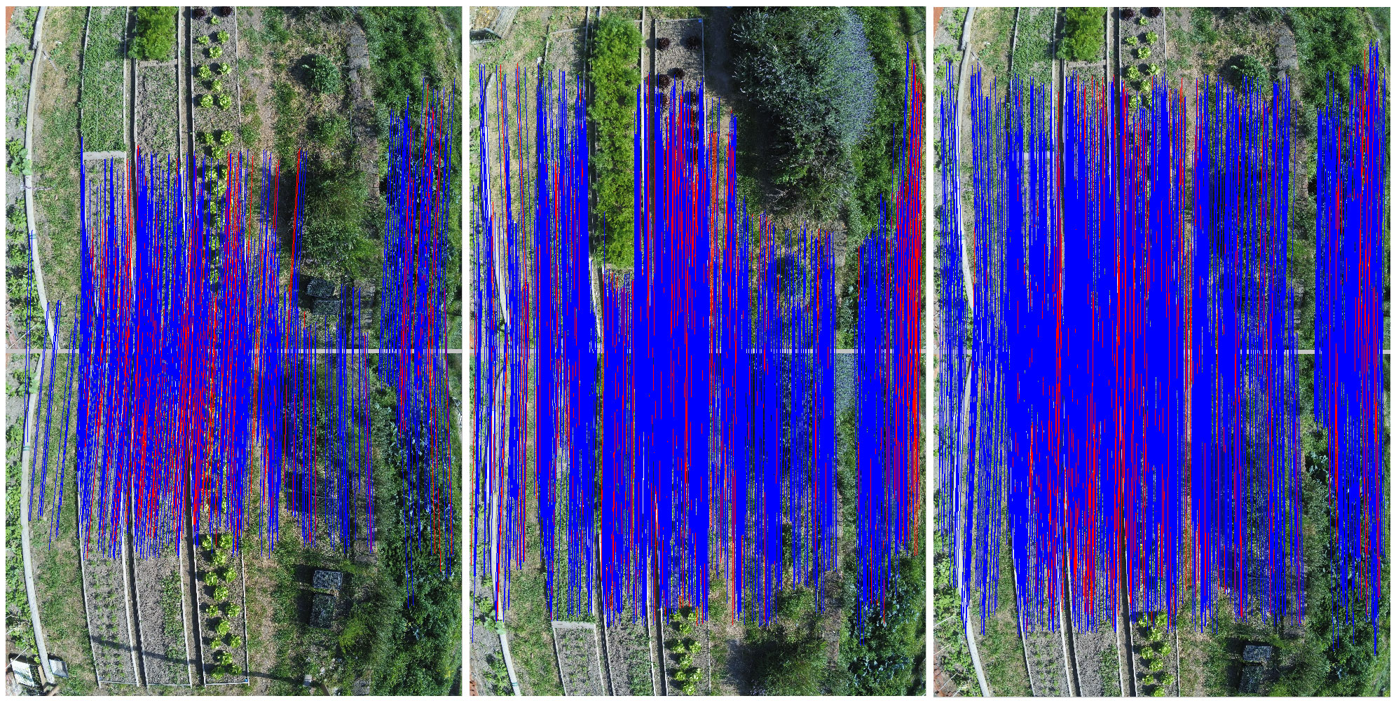
Each two pairs of images which have overlaps together are processed to find the same key points available between both (see fig 2) and following this pairing the images are geometrically corrected (orthorectified) such that the scale is uniform in all of them.

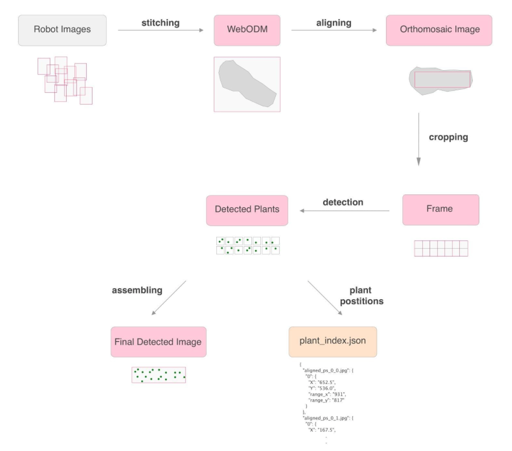
OpenDroneMap software/API was used to generate the orthomosaic image, the final outcome of this process is an aerial image of the whole crop which has a uniform scale. (see fig 3)

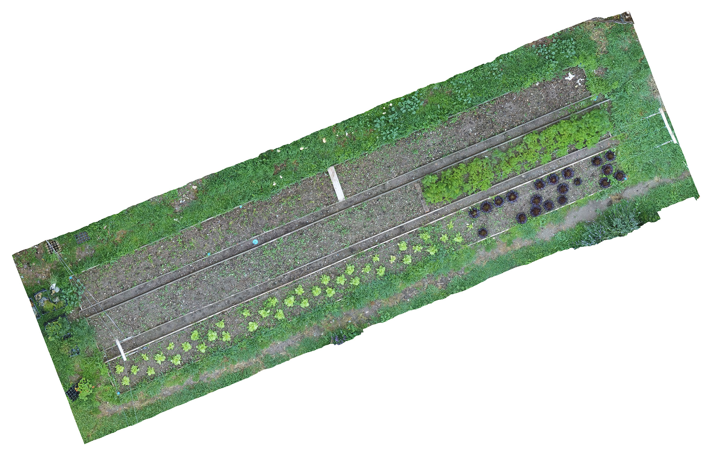
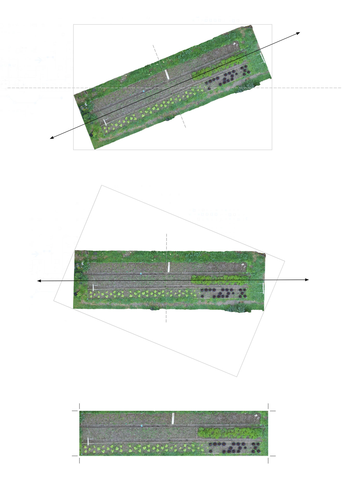
Frame Alignment Generated orthomosaic images could contain some extra parts such as extra borders, as well as random orientation. To be able to compare and analyze the maps generated from each scan overtime, we need to orient and crop them with similar boundaries and orientation. For this we include two processes of rotating the image if needed to straighten it, and as well, cropping the unnecessary parts in the borders to optimize the computation parts related to segmentation and future steps. The process of straightening the image starts by applying principal component analysis (PCA) to extract the axis line of the image, this axis line is then used to straighten the image. (see fig 4)

After aligning and cropping the orthomosaic images, they are stored in our database for the image segmentation task.

Plant Detection

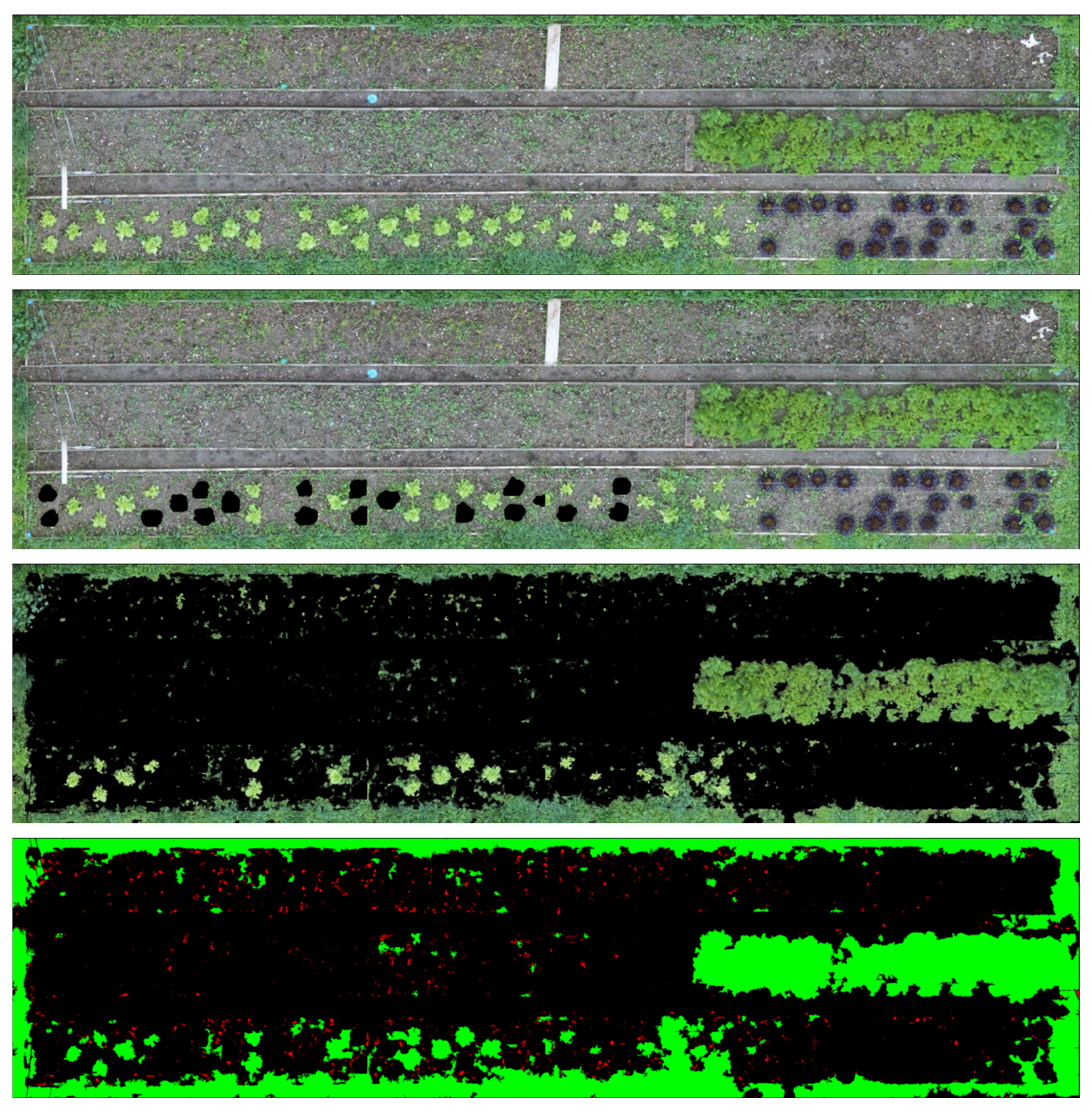
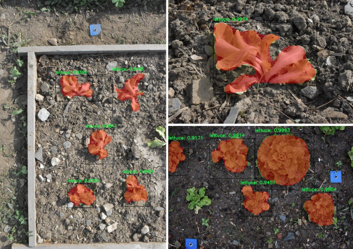
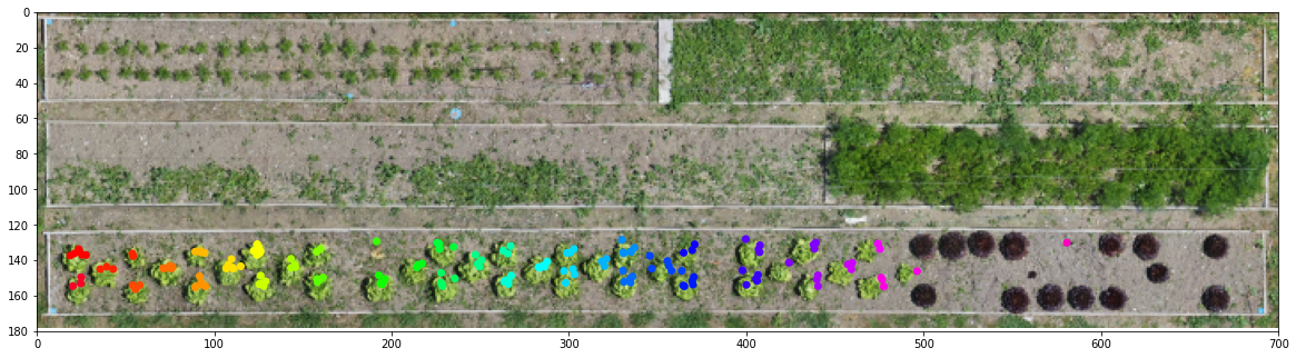
The collected orthomosaic images are generated with the pipeline explained above. In this section, we describe how the lettuces are detected and masked using Mask-RCNN, which is an instance segmentation algorithm. The generated output images show individual masks for each lettuce that is detected. The Mask-RCNN method has proven to be accurate (see the discussion of the segmentation methods in Section 1.3.6 - T6.3). This method is able to separate lettuces from different kinds of plants or weeds, as well works well with different light and shadow conditions.

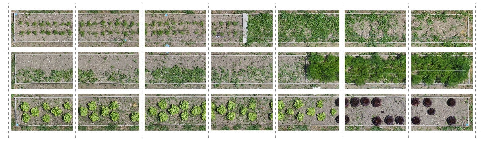
The orthomosaic images generated in step 4 are high quality large scale images. Training and Detection algorithms on these large scale images are computationally heavy therefore to apply the detection on orthomosaic images, first we divide the images to a smaller grid. The division and cell size of this grid is dependent on the crop scenario and can be defined manually by the user. The detection algorithm is applied on each cell (see Fig. 3.7).

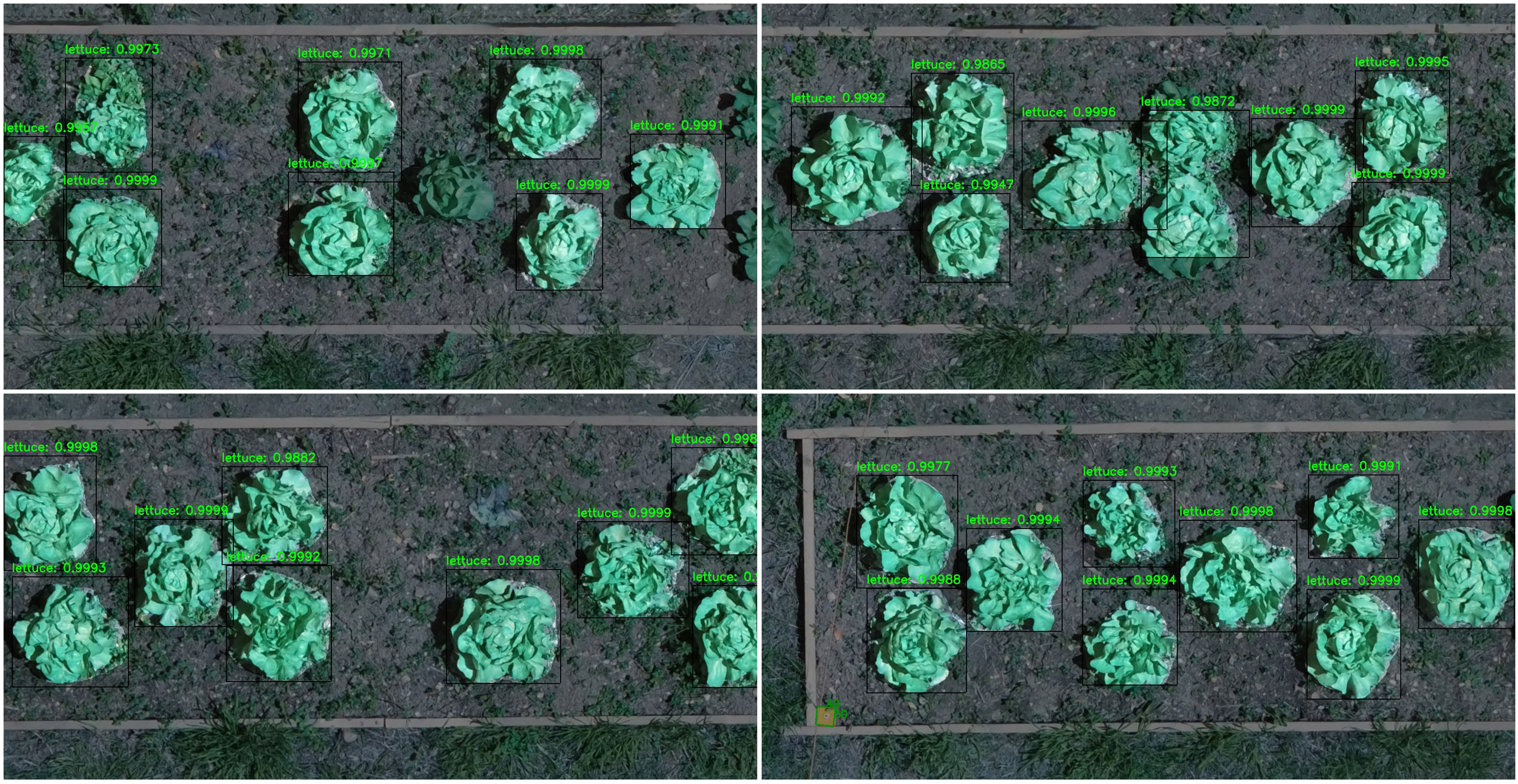
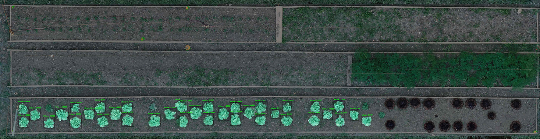
The results are merged back together to generate the overall detected image (see Fig. 3.8). In addition to the masked images, a json file containing the position and area (in the scale of image) of each detected plant is stored as well. In the next stages the masked images and the json files are used to catalog individual plants and monitor them through different scans.

Tracking Individual Plants

Once we have segmented the scan image and obtained the list of individual plants, we have to identify each plant and track each individual throughout all the scans. We tested two methods to track individual plants. In the first method, we detect each plant in each image and extract the center point of each lettuce, the centers points from each scan are then compared together with Iterative Closest Point (ICP) algorithm to track the same lettuce in different scans. In the second method, we register all maps to a common frame using feature matching and detected plants at initial growth stage. The area around each plant is then considered in all images for measuring each plant size as approximated by the projected leaf area.

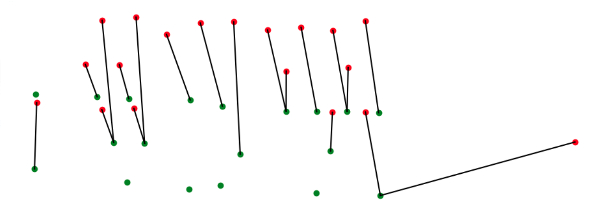
Iterative closest point algorithm on the centers of lettuces This process uses the center points of lettuces in consecutive scans for the ICP method to find the same lettuces over different scans. However, this method has two major issues.

• Undetected lettuces in some images create unmatched points
• Changes in appearance of lettuces move their center.

Registration Through Feature Matching In this process we use the position of the detected lettuces as well as the orthomosaic image generated in step 4, to track individual plants over different scans. One of the main challenges in registering and tracking individual plants in this process is to have the same frame and coordinate system for all the images. This challenge is due to two main reasons. First, the orthomosaic images have different resolutions, as well the main frame for orthomosaic images is not exactly the same for all the images. To create the same coordinate system for all the images, we use the first scan as our reference coordinate system and find the transformations between each two consecutive images using SURF feature matching methods available in OpenCV library which is based on the RANSAC algorithm. (Fig. 3.10)

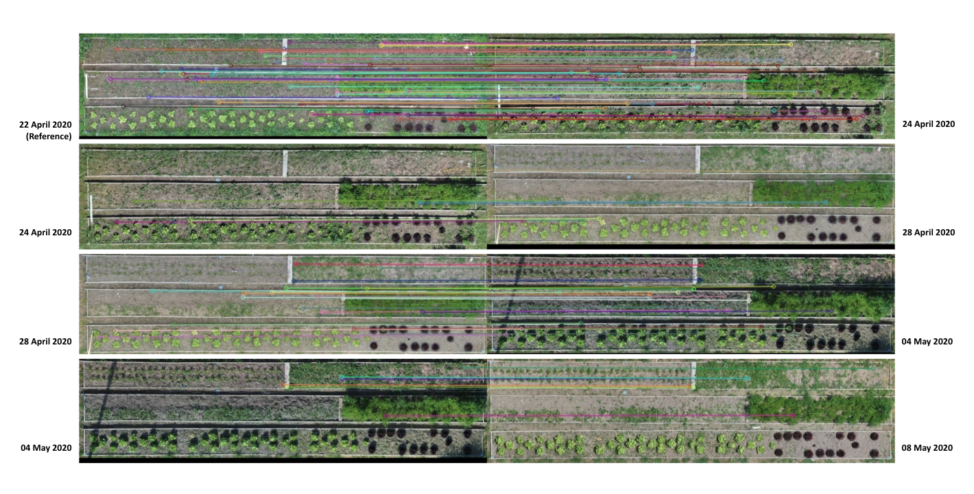
For a series of images, the transformations between each two consecutive images gets combined with all the previous transformations to calculate the transformation to our reference image (first scan). Then all the images as well as the coordinates of plants from the json file are transformed to match the same coordinate system. (see Fig. 3.11)

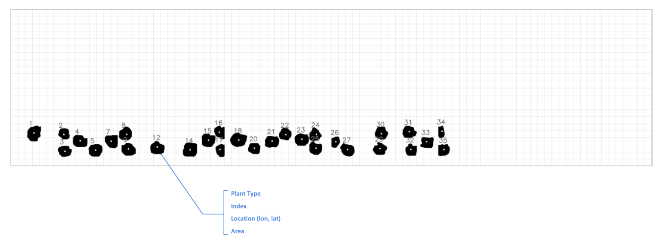
Creating a Catalog of Individual Plants

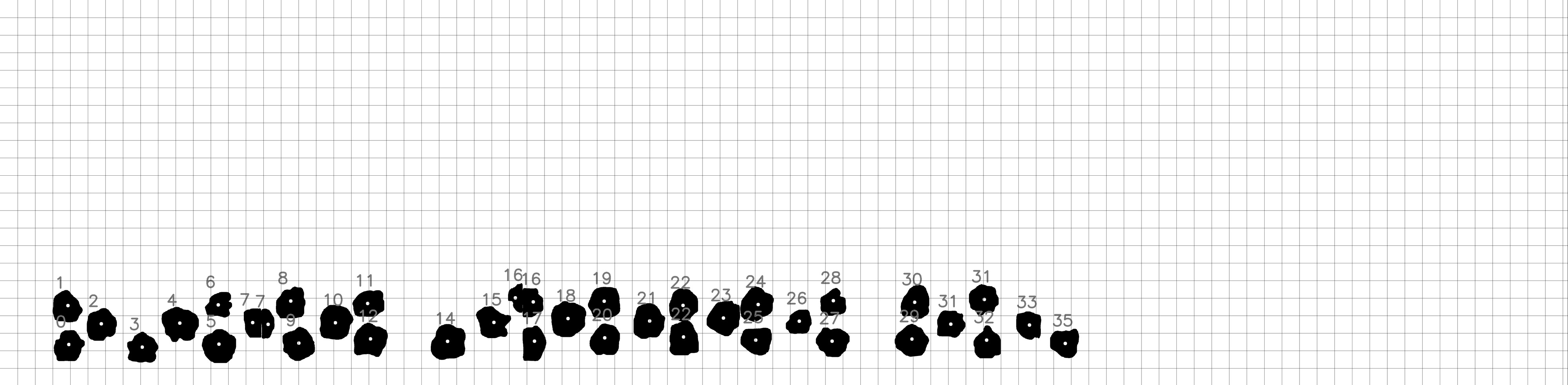
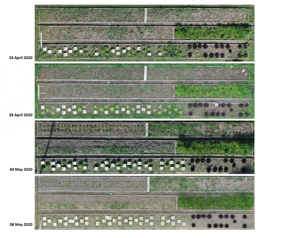
Registration of images as well as plant’s coordinates on the same coordinate system, allows for tracking of the same plant within different scans. This happens through clustering the plants’ coordinates that are within a certain distance from each other (see Fig. 3.12).

Next step is to Index the detected plant with the same ID over different scans. As well as creating a catalog of individual plants.

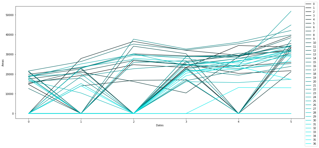
Leaf Area Monitoring and plant growth curves

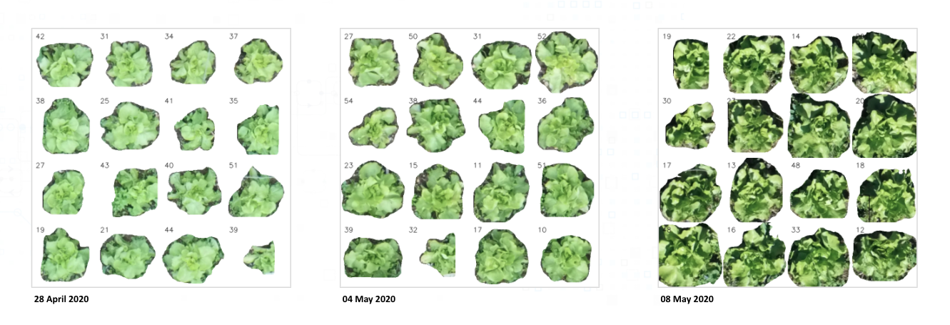
The process of registering different scans over a common reference model results in having all the coordinates and detection images in the same scale. By knowing the scale of the reference image we can scale all the images to real size world coordinates. This is crucial for extracting the leaf area from 2D images. In order to extract the leaf area we calculate the amount of detected pixels (black) over the total amount of pixels in the image which is then multiplied by the scale factor of the image. (see Fig. 3.14)

The individual leaf area extracted in each scan, is stored together with the plant’s index in a database.

Creation of weed maps

The results of the semantic segmentation can be used to map the weeds as well as the crops (Fig. 3.16). The resulting weed map provides an indicator on the areas where the pressure of the weeds is highest. These maps can be used in combination with the weeding Rover to prioritise the weeding activities.