View your results with plant-3d-explorer

How to see directly the results of your plant phenotyping with the plant-3d-explorer ?

Objective

Throughout the whole process of plant phenotyping, viewing data is often needed. This tutorial explains how to use the romi plant-3d-explorer, a web-server tool, to explore, display and interact with most of the diverse data generated during a typical plant phenotyping experiment from 2D images (2D images, 3D objects like meshes or point cloud, quality evaluations, trait measurements). After this tutorial, you should be able to:

• connect the plant-3d-explorer to a database containing the phenotyping data of one to several plants ;
• explore the database content with the plant-3d-explorer menu page ;
• For each plant, display, overlay and inspect in 3d every data generated during analysis

Prerequisite

• install romi plant-3d-explorer (from source or using a docker image ) & read install procedure
• install romi plantdb (from source or using a docker image) & read install procedure
• install romi plant-3d-vision (from source or using a docker image) & read install procedure
• Create and activate isolated python environment (see the procedure here )

Note for docker users

You can avoid installs by using docker only. Read first the docker procedures ( 'docker for plant-3d-vision' and 'docker-compose to run both database and 3d explorer with docker containers' ). In the following tutorial (steps 1, 2 and 3), follow the docker logo to adapt the procedure.

Linked documentation

• Manual of the romi plant-3d-explorer

Step-by-step tutorial

Principle: the plant-3d-explorer is a web client that displays in your favorite web browser data exposed by a server (here, romi plantdb) on a particular url. The process consists in pointing the server to your folder of interest, starting the server and starting the client that points to the served url.

Warning

the plant-3d-explorer has only been developed and tested on Chrome.

1. Preparing your database for display by the plant-3d-explorer

Starting point: your database is made of one or several datasets, which all correspond to a single plant phenotyping experiment: each dataset contains at least 2D images (raw acquisitions) and metadata, and possibly several other data generated by subsequent 3D reconstruction, segmentation and analysis.

Note

Your database must follow the rules of romi databases: please make sure that you comply to requirements. You can also download an example database here.

example: let's consider a database called my_experiment containing 3 datasets (named plant1, plant2, plant3) generated by phenotyping three plants.

• open a terminal and go to your local database directory
• if romi commands (like romi_run_task) are not accessible from your terminal, activate the appropriate python environment (e.g. using venv or conda) required for romi commands (or read this procedure)
• process all datasets for display by the plant-3d-explorer by running the following code

dataset_list=('plant1','plant2','plant3')

for ds in "${dataset_list[@]}"
do 
    romi_run_task Visualization path_to/my_experiment/"$ds"/ --config ~/configs/ml_pipe_real.toml
done

Note

For more information about using romi_run_task command, the Visualization task and the config file, please read XXXXX.

Note for docker users

• Start a docker container by mounting your database as a volume (details)
• In the container, run the same Visualization Task has above

check result: a new folder called Visualization should have been created in each dataset of your database

Note for docker users

Skip step 2 & 3 and follow instead instructions given by'docker-compose to run both database and 3d explorer with docker containers'

2. Connect your database to a local server

• Continue in the same shell terminal (if you open a new terminal, do not forget to activate appropriate python environment)
• set the DB location using the ROMI_DB environment variable
• Type the following commands to launch the server:

export ROMI_DB=/path/to/your/db
romi_scanner_rest_api #command that starts the server

check result: the terminal prints various information given by the server (e.g. number of datasets in the database). Do not stop this terminal as this will shut down the server.

3. Connect the plant-3d-explorer to the server

• Open a new terminal
• go to your local cloned directory of plant-3d-explorer/
• start the frontend visualization server by entering:

npm start

You should now be able to access the plant-3d-explorer on http://localhost:3000. Depending on you system preferences, your default web browser may automatically open a window displaying the server content. If not, open your web browser and enter http://localhost:3000 in the url bar.

Note

You need to add a file .env.local at project's root to set the API URL: REACT_APP_API_URL='{`API URL}'. Without this, the app will use: http://localhost:5000, which is the default for romi_scanner_rest_api.

4. Explore your database content via the menu page

Note

More description about the function of the menu page: read here

The starting page of the plant-3d-explorer lists the datasets of the connected database as a table and looks like this:

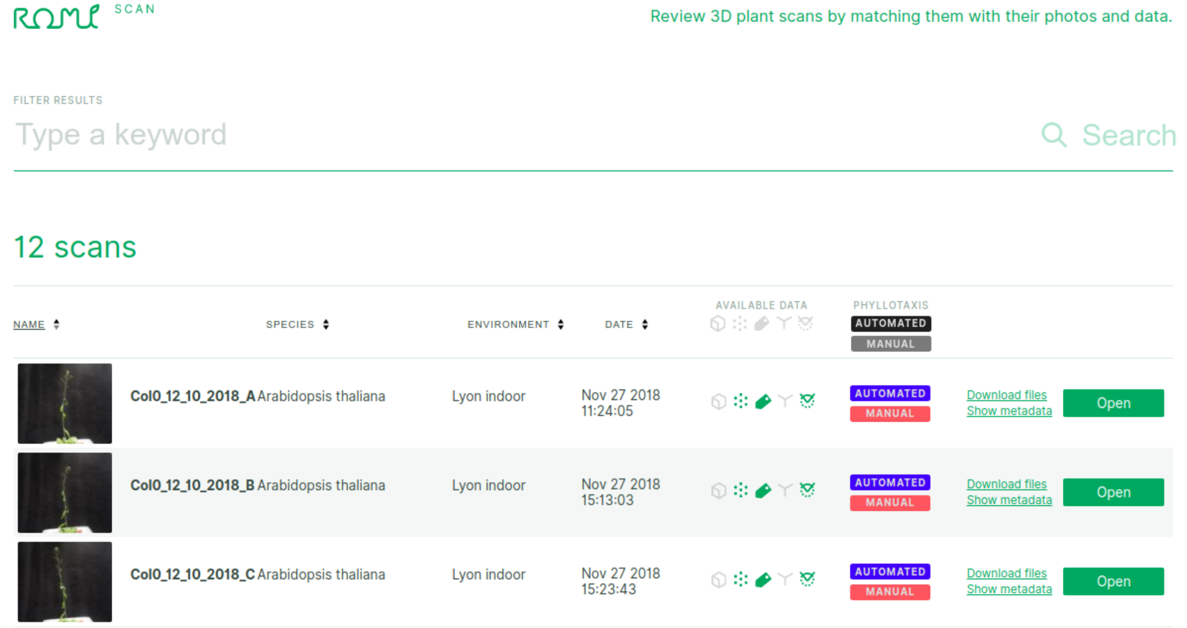
• The top search bar allows you to find particular datasets based on keywords.

• Data filters: in the header row, click on an icon to activate the filter (datasets that do not contain the data will be filtered out)

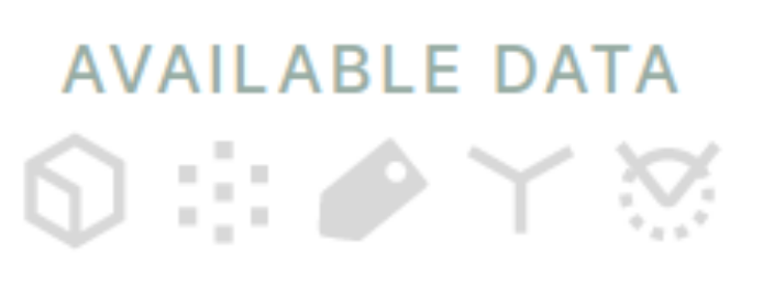  • 3d objects generated from the plant 2D images (icons respectively stand for: mesh, point cloud, segmented point cloud, skeleton and organs)

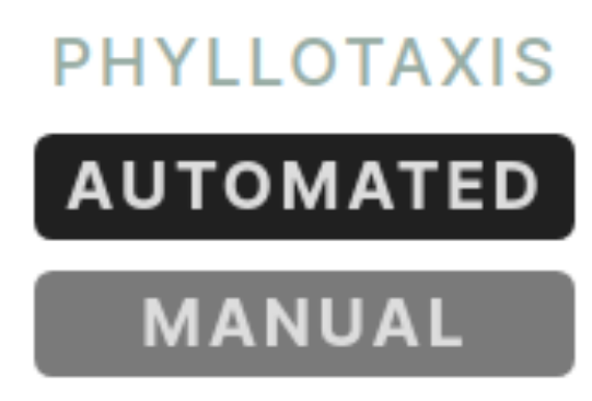  • or phyllotaxis data (manual or computed phyllotaxis measurements)

• Open a dataset with the green 'Open' button at the far right of a row

5. View a single dataset and all related data

Note

This is only a brief description to allow a quick start. More description here

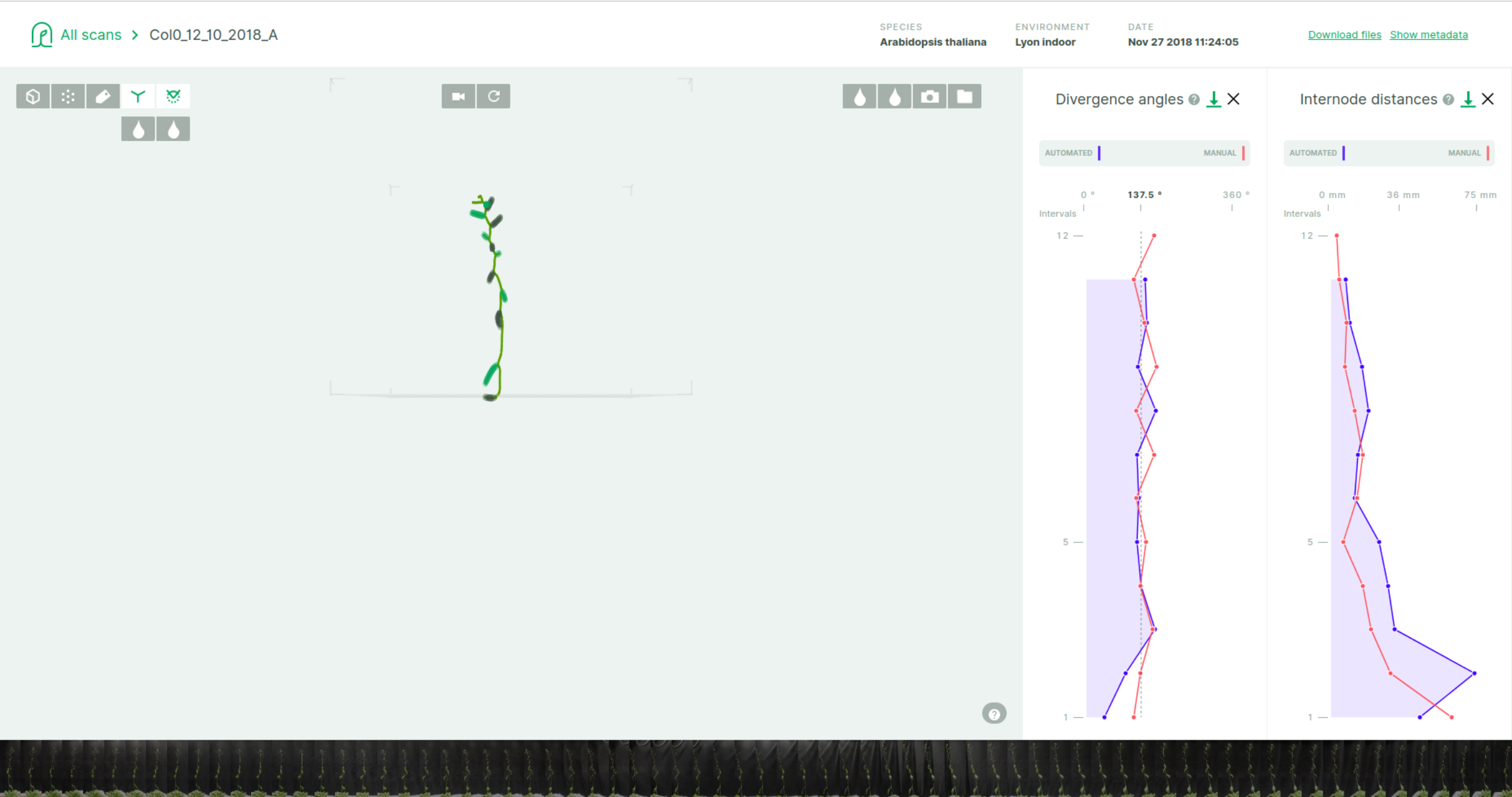
By default, the plant-3d-explorer displays in the main panel the skeleton and the organs (if available) and phyllotaxis data (as graphs) in the right panel.

Mouse-over most elements provides a brief description.

Select the 3D layers to display

In the top left corner of the main panel, icons allows you to quickly (un)select 3D layers (if available):

• White icons are active, dark grey are available but not active, light grey are not available for this dataset
• From left to right, icons represents respectively the mesh, the point-cloud, the segmented point cloud, the skeleton and the organs.

In the center of the middle panel are icons for general viewing options:

• Activate the camera icon displays the camera poses (only works if overlay with 2 images is deactivated)
• Click the round arrow to reset the view

Moving the view in the "free" 3D (without 2D overlay)

Easy movements are accessible with a mouse:

• scroll to zoom in/out
• left click rotate
• right click translate

Activate overlay with 2D images

click on any image of the bottom carousel to activate the display of 2 images in the main panel. On Mouse-over, a single picture is enlarged and proposes to open it in the main panel.

Overlay with active 3D layers is automatic. In the carousel, the box around the active displayed 2D image is now permanent.

To close the 2D overlay, just click the close button of the boxed picture in the carousel.

Moving the view with 2D overlay

Note that movement control with the mouse slightly changes compared to the "free" view without 2D overlay. Notably, the free rotation mode is not possible anymore, since it is constrained by the real movements made by the camera when it took the pictures.

• Slide right/left the active box picture in the carousel to reproduce the camera movement
• scroll to zoom in/out
• left-click to translate

The phyllotaxis measure plots

Plots represent the successive measures of divergence angles (left, in degrees) and internode length (right, in mm) between consecutive pairs of organs (here fruits) along the stem, from the base to the inflorescence tip. Both plots can be closed by clicking the cross at the far right of the plot's title. Closed plot panels can be re-opened by clicking a green "+" sign appearing at the right-hand corner when at least one plot is closed. In the plots, a blue curve correspond to "automated" measure computed through an analysis pipeline (such as pipelines developed in romi plant-3d-vision). If available in the dataset, a red curve indicates a ground-truth "manual" measure.

Mouse-over any of the two plots highlights an interval that correspond to a measure between two consecutive organs (fruits) segmented by the analysis. The interval appears synchronously on both plots if opened. This interval and the organs are numbered by their order from the base of the stem, these numbers appear on the (vertical) X-axis of the plots. The exact value of the selected interval is displayed on top of the plot ("automated" and "manual" values in blue and red respectively, if available).

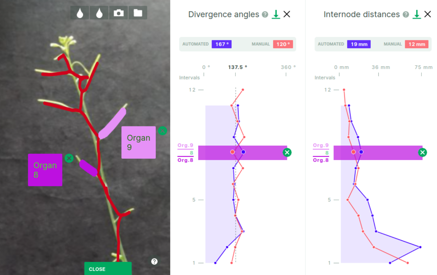
As shown above, when the 'organ' 3d-layer is active in the main panel, mouse-over the plot synchronously select the corresponding pair of organs in the current view (all other organ layers just disappear). Clicking the interval in the plot maintains the selection of the organ pair active despite further mouse movements. To deactivate the selection, click the green cross at the end of the shaded selection rectangle on either of the plots. Organ colors are also synchronized between main panel and plot panels. In the free 3D mode only, clicking a fruit layer display a bubble telling the organ number, colored as the corresponding fruit layer. Bubbles stay on screen if the 2D overlay is activated (as in the picture above).

Go back to main page

In the top left corner of the page, click "all scans":