Segmentation of images

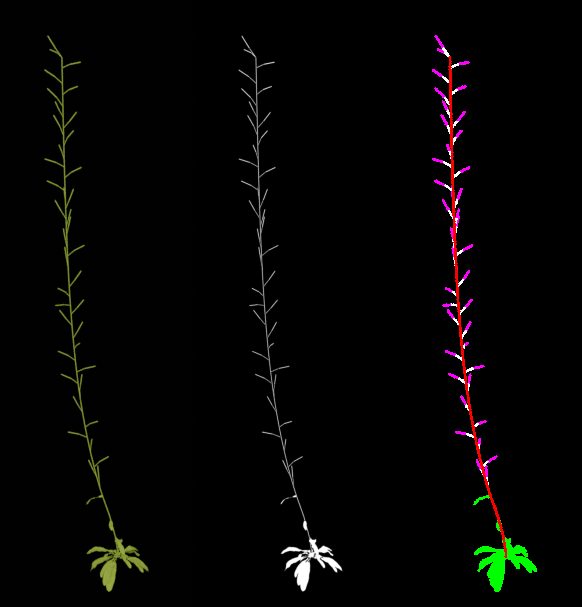
The segmentation of an image consists in assigning a label to each of its pixels. For the 3d reconstruction of a plant, we need at least the segmentation of the images into 2 classes: plant and background. For a reconstruction with semantic labeling of the point cloud, we will need a semantic segmentation of the images giving one label for each organ type (e.g. {leaf, stem,pedicel, flower, fruit}). The figure below shows the binary and multi-class segmentations for a virtual plant.

Example image of virtual arabidopsis (left) with binary (middle) and multi-class segmentation (right).

Binary segmentation

The binary segmentation of an image into plant and background is performed with the following command:

romi_run_task Masks scan_id --config myconfig.toml 

with upstream task being ImagesFilesetExists when processing the raw RGB images or Undistorded when processing images corrected using the intrinsic parameters of the camera. The task takes this set of images as an input and produce one binary mask for each image.

There are 2 methods available to compute indices for binary segmentation: Excess Green Index and Linear SVM. For each method, we provide an example configuration file in the Index computation section.

Index computation

Linear support vector machine (SVM)

A linear combination of R, G and B is used to compute the index for pixel $(i,j)$:

$$S_{ij}=w_0 R_{ij} + w_1 G_{ij} +w_2 B_{ij}$$

where $w$ is the parameters vector specified in the configuration file. A simple vector, like $w=(0,1,0)$ may be used for example.

Alternatively, you can train an SVM to learn those weights, and the threshold to be provided in the configuration file. For this, we consider you have a sample image and a ground truth binary mask. A ground truth may be produced using a manual annotation tool like LabelMe.

Using for example a list of N randomly selected pixels as $X_{train}$ (array of size [N,3]) and their corresponding labels as $Y_{train}$ (array of size N), a linear SVM is trained using

from sklearn import svm

X_train, Y_train = ...
clf = svm.SVC(kernel='linear')
clf.fit(X_train, y_train)

the weights can then be retrieved as clf.coef_ and the threshold as -clf.intercept_

Configuration file

[Masks]
upstream_task = "ImagesFilesetExists" # other option "Undistorted"
type = "linear"
parameters = "[0,1,0]"
threshold = 0.5

Excess green

This segmentation method is assuming the plant is green and the background is not. It has no parameter but it may be less robust than the linear SVM.

We compute the normalized RGB values $x \in {r,g,b}$ for each pixel $(i,j)$:

$$x_{ij} = \frac{X_{ij}}{R_{ij}+G_{ij}+B_{ij}}$$

where $X \in {R, G, B}$ is the red, green or blue image

Then, the green excess index is computed as:

$$\operatorname{ExG}=2g-r-b$$

Configuration file

[Masks]
upstream_task = "ImagesFilesetExists" # other option "Undistorted"
type = "excess_green"
threshold = 0.2

Multi-class segmentation

The Segmentation2D task performs the semantic segmentation of images using a deep neural network (DNN). The command to run this task is:

romi_run_task Segmentation2D scan_id my_config.toml

This will produce a series of binary masks, one for each class on which the network was trained.

Generic encoder/decoder architecture for semantic segmentation (U-net).

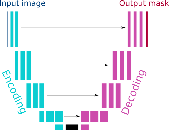
The architecture of the network is inspired from the U-net ¹, with a ResNet encoder ². It consists in encoding and decoding pathways with skip connections between the 2. Along the encoding pathways, there is a sequence of convolutions and the image signal is upsampled along the decoding pathway.

The network is trained for segmenting images of a size $(S_x,S_y)$ which is not necessarily the image size of the acquired images. Those parameters Sx and Sy should be provided in the configuration file. The images will be cropped to $(S_x,S_y)$ before being fed to the DNN and it is then resized to the original size as an output of the task.

Configuration File

[Segmentation2D]
model_id = "Resnetdataset_gl_png_896_896_epoch50"  # no default value
Sx = 896 
Sy = 896
threshold = 0.01

DNN model

The neural architecture weights are obtained through training on an annotated dataset (see How to train a DNN for semantic segmentation). Those weights should be stored in the database (at <database>/models/models) and the name of the weights file should be provided as the model_id parameter in the configuration. You can use our model trained on virtual arabidopsis here

Binarization

A binary mask $m$ is produced from the index or from the output of the DNN, I, by applying a threshold $\theta$ on I for each pixel $(i,j)$:

$$\begin{equation} m_{ij} = \begin{cases} 255 & \text{if $I_{ij}>\theta$}\\ 0 & \text{otherwise} \end{cases} \end{equation}$$

This threshold may be chosen empirically, or it may be learnt from annotated data (see linear SVM section).

Dilation

If the integer dilation parameter is non-zero a morphological dilation is applied to the image using the function binary_dilation from the skimage.morphology module.

The dilation parameter sets the number of times binary_dilation is iteratively applied. For a faithful reconstruction this parameter should be set to $0$ but in practice you may want to have a coarser point cloud. This is true when your segmentation is not perfect, dilation will fill the holes or when the reconstructed mesh is broken because the point-cloud is too thin.

Working with data from the virtual scanner

When working with data generated with the virtual scanner, the images folder contains multiple channels corresponding to the various class for which images were generated (stem, flower, fruit, leaf, pedicel). You have to select the rgb channel using the query parameter.

Configuration File

[Masks]
type = "excess_green"
threshold = 0.2
query = "{\"channel\":\"rgb\"}"

---

1. Ronneberger, O., Fischer, P., & Brox, T. (2015, October). U-net: Convolutional networks for biomedical image segmentation. In International Conference on Medical image computing and computer-assisted intervention (pp. 234-241). Springer, Cham. ↩

2. Zhang, Z., Liu, Q., & Wang, Y. (2018). Road extraction by deep residual u-net. IEEE Geoscience and Remote Sensing Letters, 15(5), 749-753. ↩